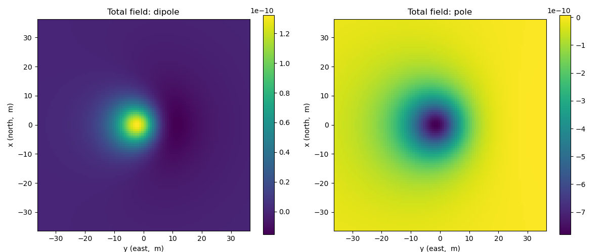
Total magnetic fields: Dipole and Pole sources

In this example, we plot anomalous total magnetic field from a magnetic dipole and pole targets. These targets are excited by Earth magnetic fields. We can vary the direction of the Earth magnetic field, and magnetic moment of the target.

author:

Seogi Kang (@sgkang)

date:

Aug 19, 2018

import numpy as np
import matplotlib.pyplot as plt
from matplotlib.colors import LogNorm
from scipy.constants import mu_0, epsilon_0

from geoana import utils, spatial
from geoana.em import static

Setup

define the location, orientation, and source, physical properties of the wholespace and source parameters

mu = mu_0  # permeability of free space (this is the default)
location = np.r_[0., 0., -10.]  # location of the dipole or pole

# dipole parameters
moment = 1
# inclination and declination (e.g. Vancouver)
inclination, declination = 67., 0.

Magnetostatic Dipole and Loop

Here, we build the geoana magnetic dipole and poie in a wholespace using the parameters defined above.

def id_to_cartesian(inclination, declination):
    ux = np.cos(inclination/180.*np.pi)*np.sin(declination/180.*np.pi)
    uy = np.cos(inclination/180.*np.pi)*np.cos(declination/180.*np.pi)
    uz = -np.sin(inclination/180.*np.pi)
    return np.r_[ux, uy, uz]

orientation = id_to_cartesian(inclination, declination)

dipole = static.MagneticDipoleWholeSpace(
    location=location,
    orientation=orientation,
    moment=moment
)

pole = static.MagneticPoleWholeSpace(
    location=location,
    orientation=orientation,
    moment=moment
)

Evaluate magnetic fields

Next, we construct a grid where we want to plot the magentic fields and evaluate

x = np.linspace(-36, 36, 100)
y = np.linspace(-36, 36, 100)
xyz = utils.ndgrid([x, y, np.r_[1.]])

# evaluate the magnetic field
b_vec_dipole = dipole.magnetic_flux_density(xyz)
b_vec_pole = pole.magnetic_flux_density(xyz)
b_total_dipole = dipole.dot_orientation(b_vec_dipole)
b_total_pole = pole.dot_orientation(b_vec_pole)

and define plotting code to plot an image of the amplitude of the vector field / flux as well as the streamlines

def plot_amplitude(ax, v):
    plt.colorbar(
        ax.pcolormesh(
            x, y, v.reshape(len(x), len(y), order='F')
        ), ax=ax
    )
    ax.axis('square')
    ax.set_xlabel('y (east,  m)')
    ax.set_ylabel('x (north,  m)')

Create subplots for plotting the results. Loop over frequencies and plot the electric and magnetic fields along a slice through the center of the dipole.

fig, ax = plt.subplots(1, 2, figsize=(12, 5))

# plot dipole vector potential
plot_amplitude(ax[0], b_total_dipole)

# plot loop vector potential
plot_amplitude(ax[1], b_total_pole)


# set the titles
ax[0].set_title("Total field: dipole")
ax[1].set_title("Total field: pole")

# format so text doesn't overlap
plt.tight_layout()
plt.show()