geoana.em.static.LineCurrentFreeSpace.magnetic_field

LineCurrentFreeSpace.magnetic_field(xyz)

Compute the magnetic field for the static current-carrying wire segments.

Parameters:

xyz(n, 3) numpy.ndarray xyz

gridded locations at which we are calculating the magnetic field

Returns:

(n, 3) numpy.ndarray

The magnetic field at each observation location in H/m.

Examples

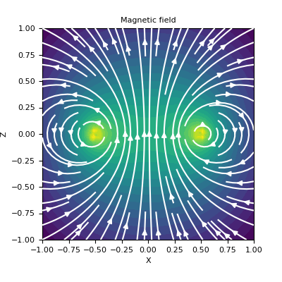
Here, we define a horizontal square loop and plot the magnetic field on the xz-plane that intercepts at y=0.

>>> from geoana.em.static import LineCurrentFreeSpace
>>> from geoana.utils import ndgrid
>>> from geoana.plotting_utils import plot2Ddata
>>> import numpy as np
>>> import matplotlib.pyplot as plt

Let us begin by defining the loop. Note that to create an inductive source, we closed the loop.

>>> x_nodes = np.array([-0.5, 0.5, 0.5, -0.5, -0.5])
>>> y_nodes = np.array([-0.5, -0.5, 0.5, 0.5, -0.5])
>>> z_nodes = np.zeros_like(x_nodes)
>>> nodes = np.c_[x_nodes, y_nodes, z_nodes]
>>> simulation = LineCurrentFreeSpace(nodes)

Now we create a set of gridded locations and compute the magnetic field.

>>> xyz = ndgrid(np.linspace(-1, 1, 50), np.array([0]), np.linspace(-1, 1, 50))
>>> H = simulation.magnetic_field(xyz)

Finally, we plot the magnetic field.

>>> fig = plt.figure(figsize=(4, 4))
>>> ax = fig.add_axes([0.15, 0.15, 0.75, 0.75])
>>> plot2Ddata(xyz[:, [0, 2]], H[:, [0, 2]], ax=ax, vec=True, scale='log', ncontour=25)
>>> ax.set_xlabel('X')
>>> ax.set_ylabel('Z')
>>> ax.set_title('Magnetic field')

(Source code, png, pdf)