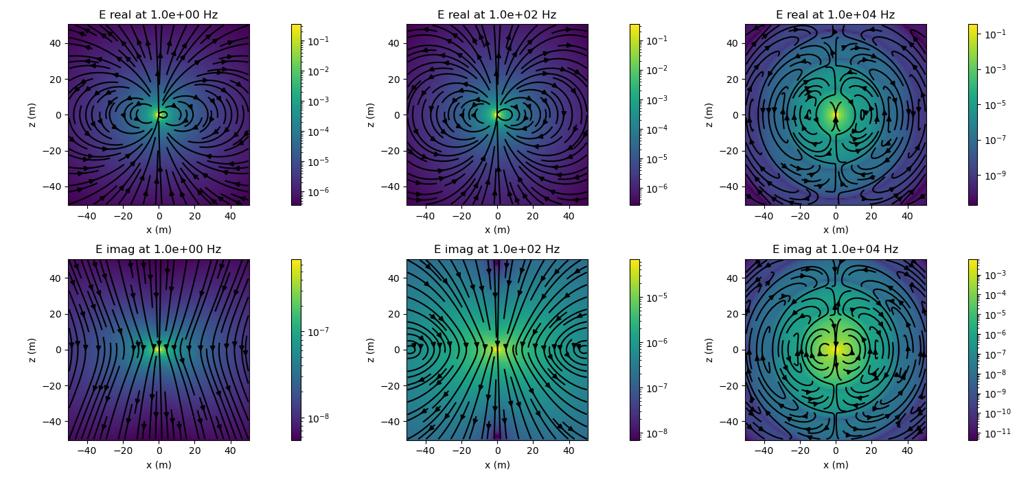
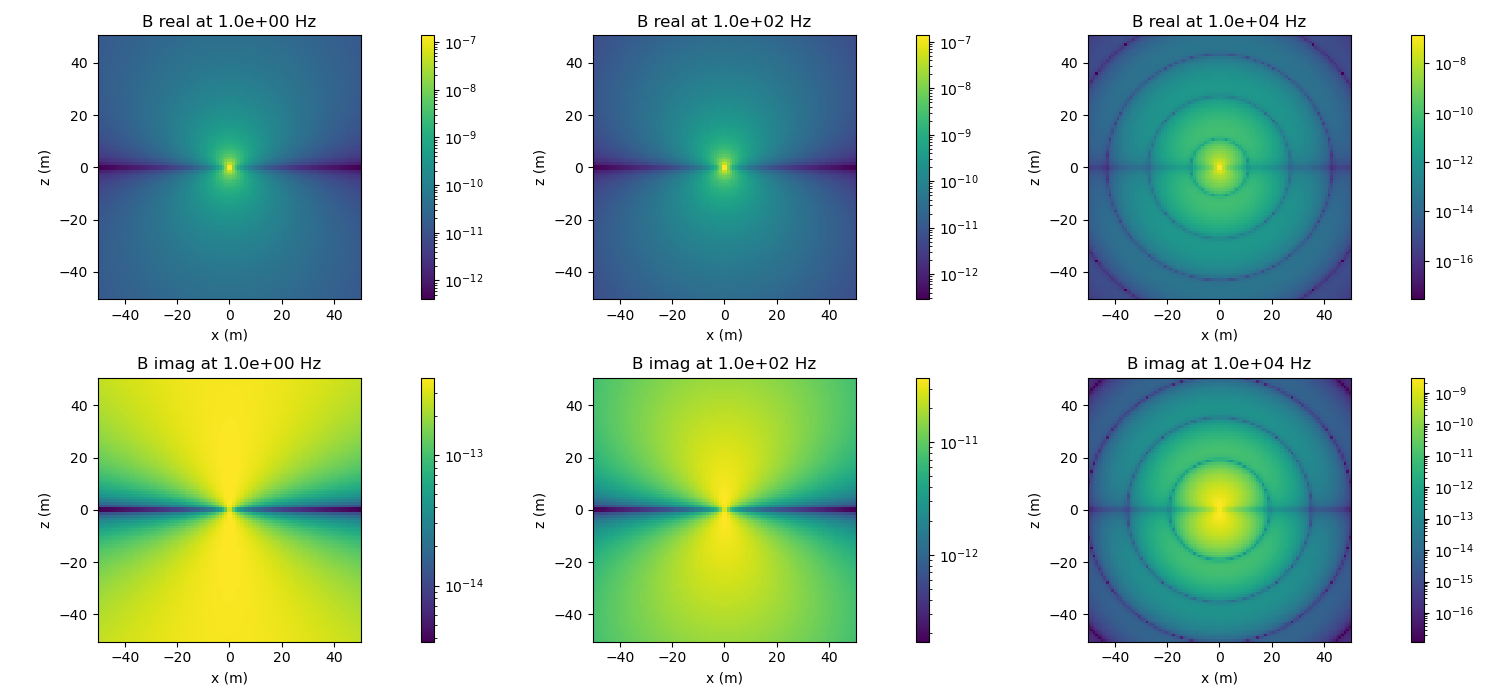
Electric Dipole in a Whole Space: Frequency Domain

In this example, we plot electric and magnetic flux density due to an electric dipole in a whole space. Note that you can also examine the current density and magnetic field.

We can vary the conductivity, magnetic permeability and dielectric permittivity of the wholespace, the frequency of the source and whether or not the quasistatic assumption is imposed.

author:

Lindsey Heagy (@lheagy)

date:

June 2, 2018

import numpy as np
import matplotlib.pyplot as plt
from matplotlib.colors import LogNorm
from scipy.constants import mu_0, epsilon_0

from geoana import utils, spatial
from geoana.em import fdem

Setup

define frequencies that we want to examine, physical properties of the wholespace and location and orientation of the dipole

frequencies = np.logspace(0, 4, 3)  # frequencies to examine
sigma = 1.  # conductivity of 1 S/m
mu = mu_0  # permeability of free space (this is the default)
epsilon=epsilon_0  # permittivity of free space (this is the default)
location=np.r_[0., 0., 0.]  # location of the dipole
orientation='Z'  # vertical dipole (can also be a unit-vector)
quasistatic=False  # don't use the quasistatic assumption

Electric Dipole

Here, we build the geoana electric dipole in a wholespace using the parameters defined above. For a full list of the properties you can set on an electric dipole, see the geoana.em.fdem.ElectricDipoleWholeSpace docs

edipole = fdem.ElectricDipoleWholeSpace(
    frequencies, sigma=sigma, mu=mu, epsilon=epsilon,
    location=location, orientation=orientation,
    quasistatic=False
)

Evaluate fields and fluxes

Next, we construct a grid where we want to plot electric fields

x = np.linspace(-50, 50, 100)
z = np.linspace(-50, 50, 100)
xyz = utils.ndgrid([x, np.r_[0], z])

and define plotting code to plot an image of the amplitude of the vector field / flux as well as the streamlines

def plot_amplitude(ax, v):
    v = spatial.vector_magnitude(v)
    plt.colorbar(
        ax.pcolormesh(
            x, z, v.reshape(len(x), len(z), order='F'), norm=LogNorm()
        ), ax=ax
    )
    ax.axis('square')
    ax.set_xlabel('x (m)')
    ax.set_ylabel('z (m)')


# plot streamlines
def plot_streamlines(ax, v):
    vx = v[:, 0].reshape(len(x), len(z), order='F')
    vz = v[:, 2].reshape(len(x), len(z), order='F')
    ax.streamplot(x, z, vx.T, vz.T, color='k')

Create subplots for plotting the results. Loop over frequencies and plot the electric and magnetic fields along a slice through the center of the dipole.

fig_e, ax_e = plt.subplots(
    2, len(frequencies), figsize=(5*len(frequencies), 7)
)
fig_b, ax_b = plt.subplots(
    2, len(frequencies), figsize=(5*len(frequencies), 7)
)

for i, frequency in enumerate(frequencies):

    # set the frequency of the dipole
    edipole.frequency = frequency

    # evaluate the electric field and magnetic flux density
    electric_field = edipole.electric_field(xyz)
    magnetic_flux_density = edipole.magnetic_flux_density(xyz)

    # plot amplitude of electric field
    for ax, reim in zip(ax_e[:, i], ['real', 'imag']):
        # grab real or imag component
        e_plot = getattr(electric_field, reim)

        # plot both amplitude and streamlines
        plot_amplitude(ax, e_plot)
        plot_streamlines(ax, e_plot)

        # set the title
        ax.set_title(
            'E {} at {:1.1e} Hz'.format(reim, frequency)
        )

    # plot the amplitude of the magnetic field (note the magnetic field is into
    # and out of the page in this geometry, so we don't plot vectors)
    for ax, reim in zip(ax_b[:, i], ['real', 'imag']):
        # grab real or imag component
        b_plot = getattr(magnetic_flux_density, reim)

        # plot amplitude
        plot_amplitude(ax, b_plot)

        # set the title
        ax.set_title(
            'B {} at {:1.1e} Hz'.format(reim, frequency)
        )

# format so text doesn't overlap
fig_e.tight_layout()
fig_b.tight_layout()
plt.show()

• 
• 

/home/runner/work/geoana/geoana/examples/em/plot_fdem_ElectricDipoleWholeSpace.py:74: UserWarning: Adding colorbar to a different Figure <Figure size 1500x700 with 7 Axes> than <Figure size 1500x700 with 6 Axes> which fig.colorbar is called on.
  plt.colorbar(
/home/runner/work/geoana/geoana/examples/em/plot_fdem_ElectricDipoleWholeSpace.py:74: UserWarning: Adding colorbar to a different Figure <Figure size 1500x700 with 8 Axes> than <Figure size 1500x700 with 6 Axes> which fig.colorbar is called on.
  plt.colorbar(
/home/runner/work/geoana/geoana/examples/em/plot_fdem_ElectricDipoleWholeSpace.py:74: UserWarning: Adding colorbar to a different Figure <Figure size 1500x700 with 9 Axes> than <Figure size 1500x700 with 8 Axes> which fig.colorbar is called on.
  plt.colorbar(
/home/runner/work/geoana/geoana/examples/em/plot_fdem_ElectricDipoleWholeSpace.py:74: UserWarning: Adding colorbar to a different Figure <Figure size 1500x700 with 10 Axes> than <Figure size 1500x700 with 8 Axes> which fig.colorbar is called on.
  plt.colorbar(
/home/runner/work/geoana/geoana/examples/em/plot_fdem_ElectricDipoleWholeSpace.py:74: UserWarning: Adding colorbar to a different Figure <Figure size 1500x700 with 11 Axes> than <Figure size 1500x700 with 10 Axes> which fig.colorbar is called on.
  plt.colorbar(
/home/runner/work/geoana/geoana/examples/em/plot_fdem_ElectricDipoleWholeSpace.py:74: UserWarning: Adding colorbar to a different Figure <Figure size 1500x700 with 12 Axes> than <Figure size 1500x700 with 10 Axes> which fig.colorbar is called on.
  plt.colorbar(