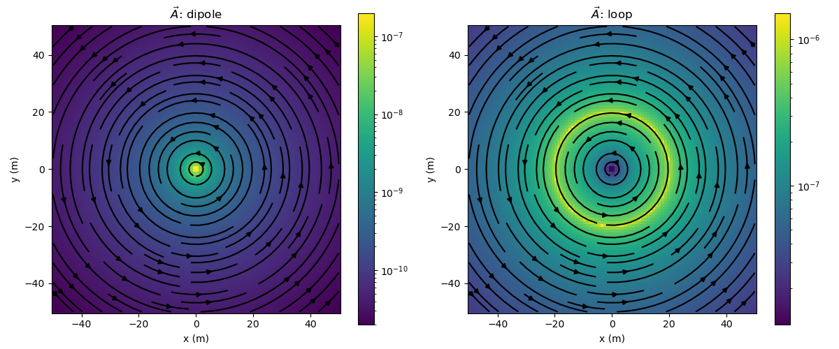
Magnetostatic Vector Potentials: Dipole and Loop Sources

In this example, we plot the vector potential for a dipole and a loop source in a wholespace.

We can vary the magnetic permeability of the wholespace, location and orientation of the sources. For the dipole source, we can vary the moment, and for the loop source, we can vary the radius and current through the loop.

author:

Lindsey Heagy (@lheagy)

date:

June 6, 2018

import numpy as np
import matplotlib.pyplot as plt
from matplotlib.colors import LogNorm
from scipy.constants import mu_0, epsilon_0

from geoana import utils, spatial
from geoana.em import static

Setup

define the location orientation and source, physical properties of the wholespace and source parameters

mu = mu_0  # permeability of free space (this is the default)
location=np.r_[0., 0., 0.]  # location of the dipole
orientation='Z'  # vertical dipole (can also be a unit-vector)

# dipole parameters
moment = 1

# loop source parameters
current = 1
radius = 20

Magnetostatic Dipole and Loop

Here, we build the geoana magnetic dipole in a wholespace and circular loop in a wholespace using the parameters defined above. For a full list of the properties you can set on a dipole, see the geoana.em.static.MagneticDipoleWholeSpace docs and for the circular loop source, see the geoana.em.static.CircularLoopWholeSpace docs

dipole = static.MagneticDipoleWholeSpace(
    mu=mu, location=location,
    orientation=orientation , moment=moment
)

loop = static.CircularLoopWholeSpace(
    mu=mu, location=location,
    orientation=orientation, current=current,
    radius=radius
)

Evaluate vector potential

Next, we construct a grid where we want to plot the vector potential and evaluate

x = np.linspace(-50, 50, 100)
y = np.linspace(-50, 50, 100)
xyz = utils.ndgrid([x, y, np.r_[0]])

# evaluate the vector potential
a_dipole = dipole.vector_potential(xyz)
a_loop = loop.vector_potential(xyz)

and define plotting code to plot an image of the amplitude of the vector field / flux as well as the streamlines

def plot_amplitude(ax, v):
    v = spatial.vector_magnitude(v)
    plt.colorbar(
        ax.pcolormesh(
            x, y, v.reshape(len(x), len(y), order='F'), norm=LogNorm()
        ), ax=ax
    )
    ax.axis('square')
    ax.set_xlabel('x (m)')
    ax.set_ylabel('y (m)')


# plot streamlines
def plot_streamlines(ax, v):
    vx = v[:, 0].reshape(len(x), len(y), order='F')
    vy = v[:, 1].reshape(len(x), len(y), order='F')
    ax.streamplot(x, y, vx.T, vy.T, color='k')

Create subplots for plotting the results. Loop over frequencies and plot the electric and magnetic fields along a slice through the center of the dipole.

fig, ax = plt.subplots(1, 2, figsize=(12, 5))

# plot dipole vector potential
plot_amplitude(ax[0], a_dipole)
plot_streamlines(ax[0], a_dipole)

# plot loop vector potential
plot_amplitude(ax[1], a_loop)
plot_streamlines(ax[1], a_loop)


# set the titles
ax[0].set_title("$\\vec{A}$: dipole")
ax[1].set_title("$\\vec{A}$: loop")

# format so text doesn't overlap
fig.tight_layout()
plt.show()