geoana.em.fdem.HarmonicPlaneWave.current_density

HarmonicPlaneWave.current_density(xyz)

Current density for the harmonic planewave at a set of gridded locations.

Parameters:

xyz(n, 3) numpy.ndarray

Gridded xyz locations

Returns:

(n_f, …, 3) numpy.ndarray of complex

Current density at all frequencies for the gridded locations provided.

Examples

Here, we define a harmonic planewave in the x-direction in a wholespace.

>>> from geoana.em.fdem import HarmonicPlaneWave
>>> import numpy as np
>>> from geoana.utils import ndgrid
>>> from mpl_toolkits.axes_grid1 import make_axes_locatable
>>> import matplotlib.pyplot as plt

Let us begin by defining the harmonic planewave in the x-direction.

>>> frequency = 1
>>> orientation = 'X'
>>> sigma = 1.0
>>> simulation = HarmonicPlaneWave(
>>>     frequency=frequency, orientation=orientation, sigma=sigma
>>> )

Now we create a set of gridded locations and compute the current density.

>>> x = np.linspace(-1, 1, 20)
>>> z = np.linspace(-1000, 0, 20)
>>> xyz = ndgrid(x, np.array([0]), z)
>>> j_vec = simulation.current_density(xyz)
>>> jx = j_vec[..., 0]
>>> jy = j_vec[..., 1]
>>> jz = j_vec[..., 2]

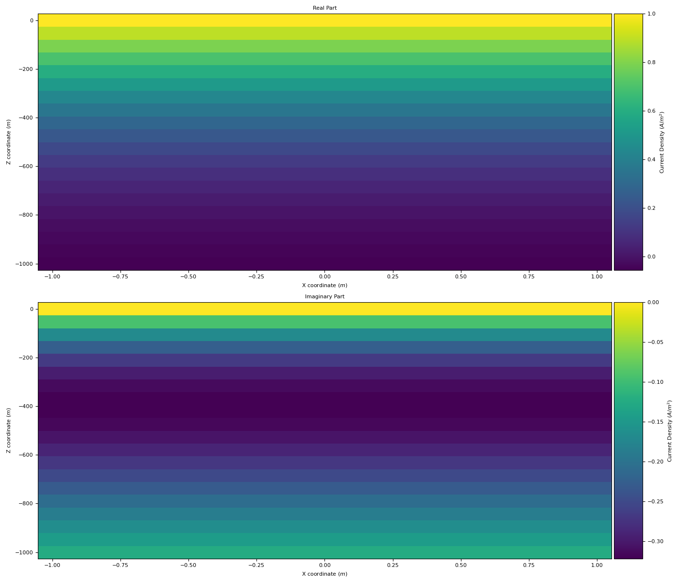
Finally, we plot the real and imaginary parts of the x-oriented current density.

>>> fig, axs = plt.subplots(2, 1, figsize=(14, 12))
>>> titles = ['Real Part', 'Imaginary Part']
>>> for ax, V, title in zip(axs.flatten(), [np.real(jx).reshape(20, 20), np.imag(jx).reshape(20, 20)], titles):
>>>     im = ax.pcolor(x, z, V, shading='auto')
>>>     divider = make_axes_locatable(ax)
>>>     cax = divider.append_axes("right", size="5%", pad=0.05)
>>>     cb = plt.colorbar(im, cax=cax)
>>>     cb.set_label(label= 'Current Density ($A/m^2$)')
>>>     ax.set_ylabel('Z coordinate ($m$)')
>>>     ax.set_xlabel('X coordinate ($m$)')
>>>     ax.set_title(title)
>>> plt.tight_layout()
>>> plt.show()

(Source code, png, pdf)