geoana.gravity.Sphere.gravitational_field

Sphere.gravitational_field(xyz)

Gravitational field due to a sphere.

\[ \begin{align}\begin{aligned}r > R\\\mathbf{g} (\mathbf{r}) = \nabla \phi (\mathbf{r})\\r < R\\\mathbf{g} (\mathbf{r}) = - \gamma \frac{4}{3} \pi \rho \mathbf{r}\end{aligned}\end{align} \]

Parameters:

xyz(…, 3) numpy.ndarray

Locations to evaluate at in units m.

Returns:

(…, 3) numpy.ndarray

Gravitational field at sphere location xyz in units \(\frac{m}{s^2}\).

Examples

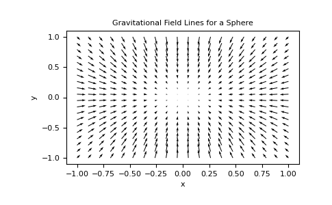
Here, we define a sphere with mass m and plot the gravitational field lines in the xy-plane.

>>> import numpy as np
>>> import matplotlib.pyplot as plt
>>> from geoana.gravity import Sphere

Define the sphere.

>>> location = np.r_[0., 0., 0.]
>>> rho = 1.0
>>> radius = 1.0
>>> simulation = Sphere(
>>>     location=location, rho=rho, radius=radius
>>> )

Now we create a set of gridded locations and compute the gravitational field.

>>> X, Y = np.meshgrid(np.linspace(-1, 1, 20), np.linspace(-1, 1, 20))
>>> Z = np.zeros_like(X) + 0.25
>>> xyz = np.stack((X, Y, Z), axis=-1)
>>> g = simulation.gravitational_field(xyz)

Finally, we plot the gravitational field lines.

>>> plt.quiver(X, Y, g[:,:,0], g[:,:,1])
>>> plt.xlabel('x')
>>> plt.ylabel('y')
>>> plt.title('Gravitational Field Lines for a Sphere')
>>> plt.show()

(Source code, png, pdf)