geoana.gravity.PointMass.gravitational_gradient

PointMass.gravitational_gradient(xyz)

Gravitational gradient for a point mass.

Parameters:

xyz(…, 3) numpy.ndarray

Observation locations in units m.

Returns:

(…, 3, 3) numpy.ndarray

Gravitational gradient at observation locations xyz in units \(\frac{1}{s^2}\).

Examples

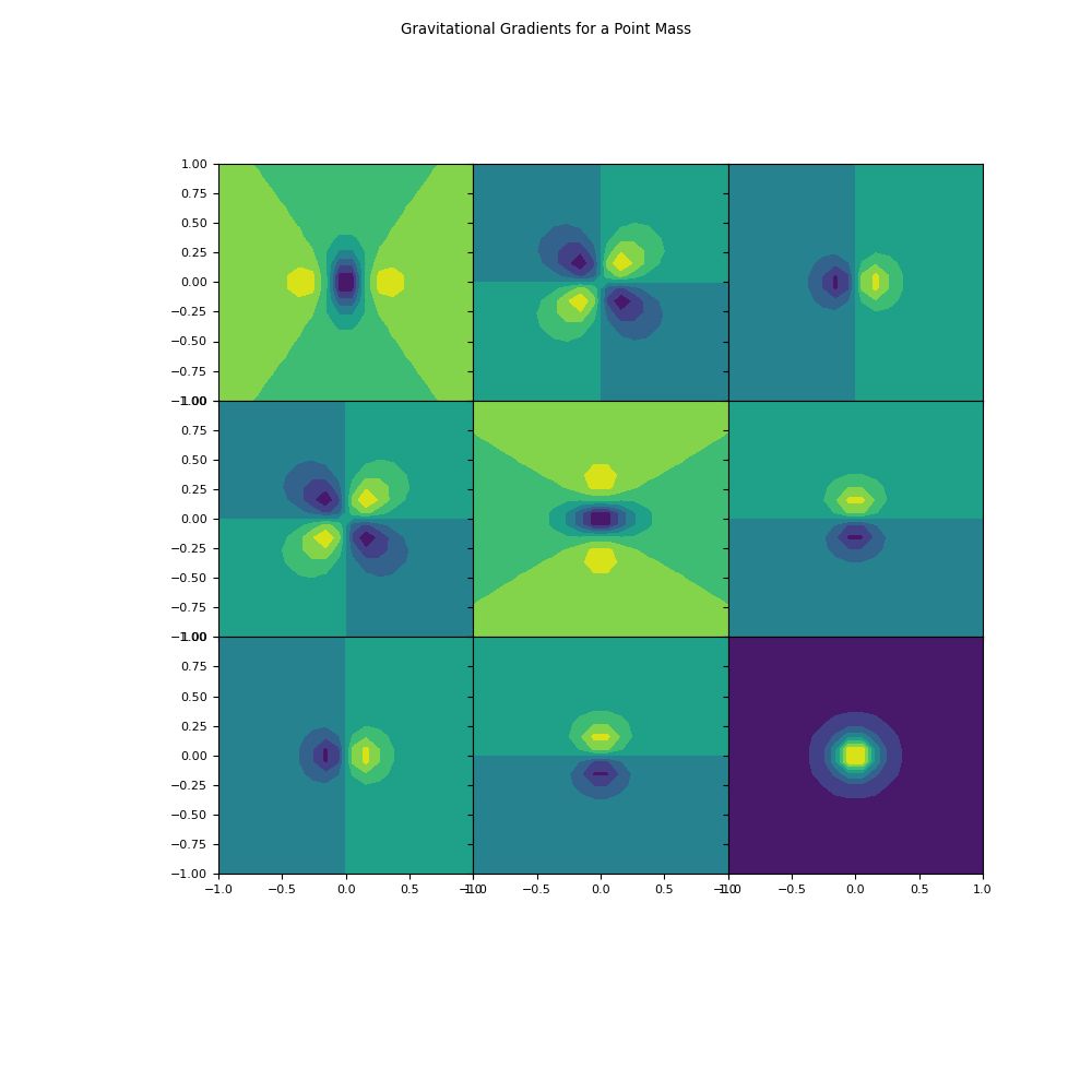
Here, we define a point mass with mass=1kg and plot the gravitational gradient.

>>> import numpy as np
>>> import matplotlib.pyplot as plt
>>> from geoana.gravity import PointMass

Define the point mass.

>>> location = np.r_[0., 0., 0.]
>>> mass = 1.0
>>> simulation = PointMass(
>>>     mass=mass, location=location
>>> )

Now we create a set of gridded locations and compute the gravitational gradient.

>>> X, Y = np.meshgrid(np.linspace(-1, 1, 20), np.linspace(-1, 1, 20))
>>> Z = np.zeros_like(X) + 0.25
>>> xyz = np.stack((X, Y, Z), axis=-1)
>>> g_tens = simulation.gravitational_gradient(xyz)

Finally, we plot the gravitational gradient for each element of the 3 x 3 matrix.

>>> fig = plt.figure(figsize=(10, 10))
>>> gs = fig.add_gridspec(3, 3, hspace=0, wspace=0)
>>> (ax1, ax2, ax3), (ax4, ax5, ax6), (ax7, ax8, ax9) = gs.subplots(sharex='col', sharey='row')
>>> fig.suptitle('Gravitational Gradients for a Point Mass')
>>> ax1.contourf(X, Y, g_tens[:,:,0,0])
>>> ax2.contourf(X, Y, g_tens[:,:,0,1])
>>> ax3.contourf(X, Y, g_tens[:,:,0,2])
>>> ax4.contourf(X, Y, g_tens[:,:,1,0])
>>> ax5.contourf(X, Y, g_tens[:,:,1,1])
>>> ax6.contourf(X, Y, g_tens[:,:,1,2])
>>> ax7.contourf(X, Y, g_tens[:,:,2,0])
>>> ax8.contourf(X, Y, g_tens[:,:,2,1])
>>> ax9.contourf(X, Y, g_tens[:,:,2,2])
>>> plt.show()

(Source code, png, pdf)