geoana.em.fdem.MagneticDipoleWholeSpace.vector_potential

MagneticDipoleWholeSpace.vector_potential(xyz)

Vector potential for the harmonic magnetic dipole at a set of gridded locations.

For a harmonic magnetic dipole oriented in the \(\hat{u}\) direction with moment amplitude \(m\), the magnetic vector potential at frequency \(f\) at vector distance \(\mathbf{r}\) from the dipole is given by:

\[\mathbf{a}(\mathbf{r}) = \frac{i \omega \mu m}{4 \pi r} e^{-ikr} \mathbf{\hat{u}}\]

where

\[k = \sqrt{\omega^2 \mu \varepsilon - i \omega \mu \sigma}\]

Parameters:

xyz(n, 3) numpy.ndarray

Gridded xyz locations

Returns:

(n_freq, n_loc, 3) numpy.array of complex

Magnetic vector potential at all frequencies for the gridded locations provided. Output array is squeezed when n_freq and/or n_loc = 1.

Examples

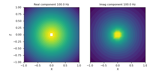
Here, we define an z-oriented magnetic dipole and plot the magnetic vector potential on the xy-plane that intercepts z=0.

>>> from geoana.em.fdem import MagneticDipoleWholeSpace
>>> from geoana.utils import ndgrid
>>> from geoana.plotting_utils import plot2Ddata
>>> import numpy as np
>>> import matplotlib.pyplot as plt

Let us begin by defining the electric current dipole.

>>> frequency = np.logspace(1, 3, 3)
>>> location = np.r_[0., 0., 0.]
>>> orientation = np.r_[0., 0., 1.]
>>> moment = 1.
>>> sigma = 1.0
>>> simulation = MagneticDipoleWholeSpace(
>>>     frequency, location=location, orientation=orientation,
>>>     moment=moment, sigma=sigma
>>> )

Now we create a set of gridded locations and compute the vector potential.

>>> xyz = ndgrid(np.linspace(-1, 1, 20), np.linspace(-1, 1, 20), np.array([0]))
>>> a = simulation.vector_potential(xyz)

Finally, we plot the real and imaginary components of the vector potential.

>>> f_ind = 1
>>> fig = plt.figure(figsize=(6, 3))
>>> ax1 = fig.add_axes([0.15, 0.15, 0.40, 0.75])
>>> plot2Ddata(xyz[:, 0:2], np.real(a[f_ind, :, 2]), ax=ax1, scale='log', ncontour=25)
>>> ax1.set_xlabel('X')
>>> ax1.set_ylabel('Z')
>>> ax1.autoscale(tight=True)
>>> ax1.set_title('Real component {} Hz'.format(frequency[f_ind]))
>>> ax2 = fig.add_axes([0.6, 0.15, 0.40, 0.75])
>>> plot2Ddata(xyz[:, 0:2], np.imag(a[f_ind, :, 2]), ax=ax2, scale='log', ncontour=25)
>>> ax2.set_xlabel('X')
>>> ax2.set_yticks([])
>>> ax2.autoscale(tight=True)
>>> ax2.set_title('Imag component {} Hz'.format(frequency[f_ind]))

(Source code, png, pdf)