geoana.em.fdem.MagneticDipoleHalfSpace.magnetic_field

MagneticDipoleHalfSpace.magnetic_field(xy, field='secondary')

Magnetic field due to a magnetic dipole over a half space

The analytic expression is only valid for a source and receiver at the surface of the earth. For arbitrary source and receiver locations above the earth, use the layered solution.

Parameters:

xy(…, 2) numpy.ndarray

receiver locations of shape

field(“secondary”, “total”)

Flag for the type of field to return.

Returns:

(n_freq, …, 3) numpy.array of complex

Magnetic field at all frequencies for the gridded locations provided. Output array is squeezed when n_freq and/or n_loc = 1.

Examples

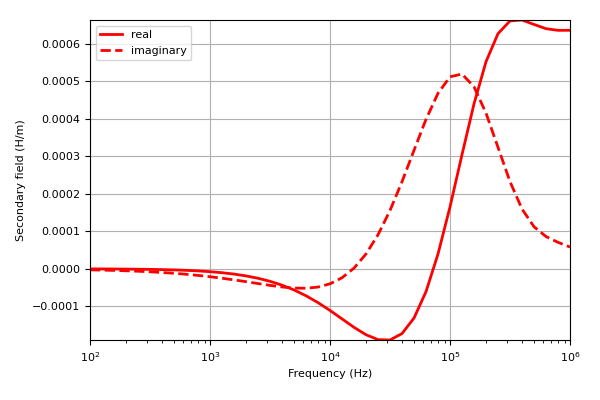
Here, we define an z-oriented magnetic dipole at (0, 0, 0) and plot the secondary magnetic field at multiple frequencies at (5, 0, 0).

>>> from geoana.em.fdem import MagneticDipoleHalfSpace
>>> from geoana.utils import ndgrid
>>> from geoana.plotting_utils import plot2Ddata
>>> import numpy as np
>>> import matplotlib.pyplot as plt

Let us begin by defining the electric current dipole.

>>> frequency = np.logspace(2, 6, 41)
>>> location = np.r_[0., 0., 0.]
>>> orientation = np.r_[0., 0., 1.]
>>> moment = 1.
>>> sigma = 1.0
>>> simulation = MagneticDipoleHalfSpace(
>>>     frequency, location=location, orientation=orientation,
>>>     moment=moment, sigma=sigma
>>> )

Now we define the receiver location and plot the secondary field.

>>> xyz = np.c_[5, 0, 0]
>>> H = simulation.magnetic_field(xyz, field='secondary')

Finally, we plot the real and imaginary components of the magnetic field.

>>> fig = plt.figure(figsize=(6, 4))
>>> ax1 = fig.add_axes([0.15, 0.15, 0.8, 0.8])
>>> ax1.semilogx(frequency, np.real(H[:, 2]), 'r', lw=2)
>>> ax1.semilogx(frequency, np.imag(H[:, 2]), 'r--', lw=2)
>>> ax1.set_xlabel('Frequency (Hz)')
>>> ax1.set_ylabel('Secondary field (H/m)')
>>> ax1.grid()
>>> ax1.autoscale(tight=True)
>>> ax1.legend(['real', 'imaginary'])

(Source code, png, pdf)