geoana.em.static.MagneticDipoleWholeSpace.vector_potential

MagneticDipoleWholeSpace.vector_potential(xyz, coordinates='cartesian')

Compute the vector potential for the static magnetic dipole.

This method computes the vector potential for the magnetic dipole at the set of gridded xyz locations provided. Where \(\mu\) is the magnetic permeability, \(\mathbf{m}\) is the dipole moment, \(\mathbf{r_0}\) the dipole location and \(\mathbf{r}\) is the location at which we want to evaluate the vector potential \(\mathbf{a}\):

\[\mathbf{a}(\mathbf{r}) = \frac{\mu}{4\pi} \frac{\mathbf{m} \times \, \Delta \mathbf{r}}{| \Delta r |^3}\]

where

\[\mathbf{\Delta r} = \mathbf{r} - \mathbf{r_0}\]

For reference, see equation 5.83 in Griffiths (1999).

Parameters:

xyz(n, 3) numpy.ndarray xyz

gridded locations at which we are calculating the vector potential

coordinates: str {‘cartesian’, ‘cylindrical’}

coordinate system that the location (xyz) are provided. The solution is also returned in this coordinate system. Default: “cartesian”

Returns:

(n, 3) numpy.ndarray

The magnetic vector potential at each observation location in the coordinate system specified in units Tm.

Examples

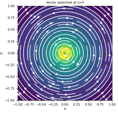
Here, we define a z-oriented magnetic dipole and plot the vector potential on the xy-plane that intercepts at z=0.

>>> from geoana.em.static import MagneticDipoleWholeSpace
>>> from geoana.utils import ndgrid
>>> from geoana.plotting_utils import plot2Ddata
>>> import numpy as np
>>> import matplotlib.pyplot as plt

Let us begin by defining the magnetic dipole.

>>> location = np.r_[0., 0., 0.]
>>> orientation = np.r_[0., 0., 1.]
>>> moment = 1.
>>> dipole_object = MagneticDipoleWholeSpace(
>>>     location=location, orientation=orientation, moment=moment
>>> )

Now we create a set of gridded locations and compute the vector potential.

>>> xyz = ndgrid(np.linspace(-1, 1, 20), np.linspace(-1, 1, 20), np.array([0]))
>>> a = dipole_object.vector_potential(xyz)

Finally, we plot the vector potential on the plane. Given the symmetry, there are only horizontal components.

>>> fig = plt.figure(figsize=(4, 4))
>>> ax = fig.add_axes([0.15, 0.15, 0.8, 0.8])
>>> plot2Ddata(xyz[:, 0:2], a[:, 0:2], ax=ax, vec=True, scale='log')
>>> ax.set_xlabel('X')
>>> ax.set_ylabel('Z')
>>> ax.set_title('Vector potential at z=0')

(Source code, png, pdf)