geoana.em.static.CircularLoopWholeSpace.vector_potential

CircularLoopWholeSpace.vector_potential(xyz, coordinates='cartesian')

Compute the vector potential for the static loop in a wholespace.

This method computes the vector potential for the cirular current loop at the set of gridded xyz locations provided. Where \(\mu\) is the magnetic permeability, \(I d\mathbf{s}\) represents an infinitessimal segment of current at location \(\mathbf{r_s}\) and \(\mathbf{r}\) is the location at which we want to evaluate the vector potential \(\mathbf{a}\):

\[\mathbf{a}(\mathbf{r}) = \frac{\mu I}{4\pi} \oint \frac{1}{|\mathbf{r} - \mathbf{r_s}|} d\mathbf{s}\]

The above expression can be solve analytically by using the appropriate change of coordinate transforms and the solution for a horizontal current loop. For a horizontal current loop centered at (0,0,0), the solution in radial coordinates is given by:

\[a_\theta (\rho, z) = \frac{\mu_0 I}{\pi k} \sqrt{ \frac{R}{\rho^2}} \bigg [ (1 - k^2/2) \, K(k^2) - K(k^2) \bigg ]\]

where

\[k^2 = \frac{4 R \rho}{(R + \rho)^2 + z^2}\]

and

• \(\rho = \sqrt{x^2 + y^2}\) is the horizontal distance to the test point

• \(I\) is the current through the loop

• \(R\) is the radius of the loop

• \(E(k^2)\) and \(K(k^2)\) are the complete elliptic integrals

Parameters:

xyz(n, 3) numpy.ndarray xyz

gridded locations at which we calculate the vector potential

coordinates: str {‘cartesian’, ‘cylindrical’}

coordinate system that the location (xyz) are provided. The solution is also returned in this coordinate system. Default: “cartesian”

Returns:

(n, 3) numpy.ndarray

The magnetic vector potential at each observation location in the coordinate system specified in units Tm.

Examples

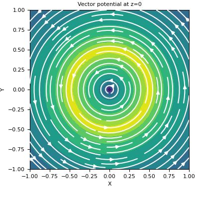
Here, we define a horizontal loop and plot the vector potential on the xy-plane that intercepts at z=0.

>>> from geoana.em.static import CircularLoopWholeSpace
>>> from geoana.utils import ndgrid
>>> from geoana.plotting_utils import plot2Ddata
>>> import numpy as np
>>> import matplotlib.pyplot as plt

Let us begin by defining the loop.

>>> location = np.r_[0., 0., 0.]
>>> orientation = np.r_[0., 0., 1.]
>>> radius = 0.5
>>> simulation = CircularLoopWholeSpace(
>>>     location=location, orientation=orientation, radius=radius
>>> )

Now we create a set of gridded locations and compute the vector potential.

>>> xyz = ndgrid(np.linspace(-1, 1, 50), np.linspace(-1, 1, 50), np.array([0]))
>>> a = simulation.vector_potential(xyz)

Finally, we plot the vector potential on the plane. Given the symmetry, there are only horizontal components.

>>> fig = plt.figure(figsize=(4, 4))
>>> ax = fig.add_axes([0.15, 0.15, 0.8, 0.8])
>>> plot2Ddata(xyz[:, 0:2], a[:, 0:2], ax=ax, vec=True, scale='log')
>>> ax.set_xlabel('X')
>>> ax.set_ylabel('Y')
>>> ax.set_title('Vector potential at z=0')

(Source code, png, pdf)