geoana.em.tdem.vertical_magnetic_field_time_deriv_horizontal_loop

geoana.em.tdem.vertical_magnetic_field_time_deriv_horizontal_loop(t, sigma=1.0, mu=1.25663706212e-06, radius=1.0, current=1.0, turns=1)

Time-derivative of the vertical transient magnetic field at the center of a horizontal loop over a halfspace.

Compute the time-derivative of the vertical component of the transient magnetic field at the center of a circular loop on the surface of a conductive and magnetically permeable halfspace.

Parameters:

tfloat, or numpy.ndarray

sigmafloat, optional

conductivity

mufloat, optional

magnetic permeability

radiusfloat, optional

radius of the horizontal loop

currentfloat, optional

current of the horizontal loop

turnsint, optional

number of turns in the horizontal loop

Returns:

dhz_dtfloat, or numpy.ndarray

The vertical magnetic field time derivative at the center of the loop. The shape will match the t input.

Notes

Matches equation 4.97 of Ward and Hohmann 1988.

\[\frac{\partial h_z}{\partial t} = -\frac{I}{\sigma a^3}\left[ 3 \mathrm{erf}(\theta a) - \frac{2}{\sqrt{\pi}}\theta a (3 + 2 \theta^2 a^2)e^{-\theta^2 a^2} \right]\]

Examples

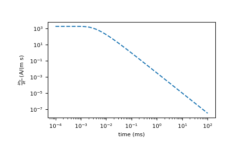
Reproducing part of Figure 4.8 from Ward and Hohmann 1988

>>> import numpy as np
>>> import matplotlib.pyplot as plt
>>> from geoana.em.tdem import vertical_magnetic_field_time_deriv_horizontal_loop

Calculate the field at the time given

>>> times = np.logspace(-7, -1)
>>> dhz_dt = vertical_magnetic_field_time_deriv_horizontal_loop(times, sigma=1E-2, radius=50)

Match the vertical magnetic field plot

>>> plt.loglog(times*1E3, -dhz_dt, '--')
>>> plt.xlabel('time (ms)')
>>> plt.ylabel(r'$\frac{\partial h_z}{ \partial t}$ (A/(m s)')
>>> plt.show()

(Source code, png, pdf)