geoana.em.static.ElectrostaticSphere.current_density

ElectrostaticSphere.current_density(xyz, field='all')

Current density for a sphere in a uniform wholespace

Parameters:

xyz(…, 3) numpy.ndarray

Locations to evaluate at in units m.

field{‘all’, ‘total’, ‘primary’, ‘secondary’}

Returns:

Jt, Jp, Js(…, 3) np.ndarray

If field == “all”

J(…, 3) np.ndarray

If only requesting a single field.

Examples

Here, we define a sphere with conductivity sigma_sphere in a uniform electrostatic field with conductivity sigma_background and plot the total and secondary current densities.

>>> import numpy as np
>>> import matplotlib.pyplot as plt
>>> from matplotlib import patches
>>> from mpl_toolkits.axes_grid1 import make_axes_locatable
>>> from geoana.em.static import ElectrostaticSphere

Define the sphere.

>>> sigma_sphere = 10. ** -1
>>> sigma_background = 10. ** -3
>>> radius = 1.0
>>> simulation = ElectrostaticSphere(
>>>     location=None, sigma_sphere=sigma_sphere, sigma_background=sigma_background, radius=radius, primary_field=None
>>> )

Now we create a set of gridded locations and compute the current densities.

>>> X, Y = np.meshgrid(np.linspace(-2*radius, 2*radius, 20), np.linspace(-2*radius, 2*radius, 20))
>>> Z = np.zeros_like(X) + 0.25
>>> xyz = np.stack((X, Y, Z), axis=-1)
>>> jt = simulation.current_density(xyz, field='total')
>>> js = simulation.current_density(xyz, field='secondary')

Finally, we plot the total and secondary current densities.

>>> fig, axs = plt.subplots(1, 2, figsize=(18,12))
>>> titles = ['Total Current Density', 'Secondary Current Density']
>>> for ax, J, title in zip(axs.flatten(), [jt, js], titles):
>>>     J_amp = np.linalg.norm(J, axis=-1)
>>>     im = ax.pcolor(X, Y, J_amp, shading='auto')
>>>     divider = make_axes_locatable(ax)
>>>     cax = divider.append_axes("right", size="5%", pad=0.05)
>>>     cb = plt.colorbar(im, cax=cax)
>>>     cb.set_label(label= 'Current Density ($A/m^2$)')
>>>     ax.streamplot(X, Y, J[..., 0], J[..., 1], density=0.75)
>>>     ax.add_patch(patches.Circle((0, 0), radius, fill=False, linestyle='--'))
>>>     ax.set_ylabel('Y coordinate ($m$)')
>>>     ax.set_xlabel('X coordinate ($m$)')
>>>     ax.set_aspect('equal')
>>>     ax.set_title(title)
>>> plt.tight_layout()
>>> plt.show()

(Source code, png, pdf)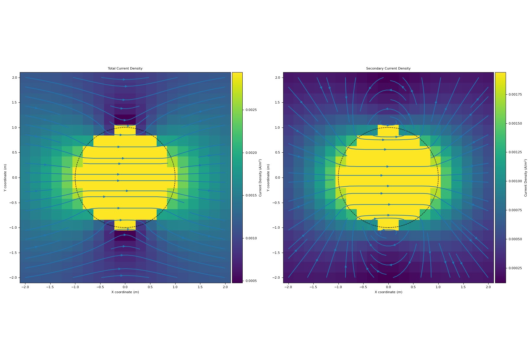