geoana.em.static.MagneticDipoleWholeSpace.magnetic_field

MagneticDipoleWholeSpace.magnetic_field(xyz, coordinates='cartesian')

Compute the magnetic field produced by a static magnetic dipole.

This method computes the magnetic field produced by the static magnetic dipole at the set of gridded xyz locations provided. Where \(\mathbf{m}\) is the dipole moment, \(\mathbf{r_0}\) is the dipole location and \(\mathbf{r}\) is the location at which we want to evaluate the magnetic field \(\mathbf{H}\):

\[\mathbf{H}(\mathbf{r}) = \frac{1}{4\pi} \Bigg [ \frac{3 \Delta \mathbf{r} \big ( \mathbf{m} \cdot \, \Delta \mathbf{r} \big ) }{| \Delta \mathbf{r} |^5} - \frac{\mathbf{m}}{| \Delta \mathbf{r} |^3} \Bigg ]\]

where

\[\mathbf{\Delta r} = \mathbf{r} - \mathbf{r_0}\]

For reference, see equation Griffiths (1999).

Parameters:

xyz(n, 3) numpy.ndarray xyz

gridded locations at which we calculate the magnetic field

coordinates: str {‘cartesian’, ‘cylindrical’}

coordinate system that the location (xyz) are provided. The solution is also returned in this coordinate system. Default: “cartesian”

Returns:

(n, 3) numpy.ndarray

The magnetic field at each observation location in the coordinate system specified in units A/m.

Examples

Here, we define a z-oriented magnetic dipole and plot the magnetic field on the xz-plane that intercepts y=0.

>>> from geoana.em.static import MagneticDipoleWholeSpace
>>> from geoana.utils import ndgrid
>>> from geoana.plotting_utils import plot2Ddata
>>> import numpy as np
>>> import matplotlib.pyplot as plt

Let us begin by defining the magnetic dipole.

>>> location = np.r_[0., 0., 0.]
>>> orientation = np.r_[0., 0., 1.]
>>> moment = 1.
>>> dipole_object = MagneticDipoleWholeSpace(
>>>     location=location, orientation=orientation, moment=moment
>>> )

Now we create a set of gridded locations and compute the vector potential.

>>> xyz = ndgrid(np.linspace(-1, 1, 20), np.array([0]), np.linspace(-1, 1, 20))
>>> H = dipole_object.magnetic_field(xyz)

Finally, we plot the vector potential on the plane. Given the symmetry, there are only horizontal components.

>>> fig = plt.figure(figsize=(4, 4))
>>> ax = fig.add_axes([0.15, 0.15, 0.8, 0.8])
>>> plot2Ddata(xyz[:, 0::2], H[:, 0::2], ax=ax, vec=True, scale='log')
>>> ax.set_xlabel('X')
>>> ax.set_ylabel('Z')
>>> ax.set_title('Magnetic field at y=0')

(Source code, png, pdf)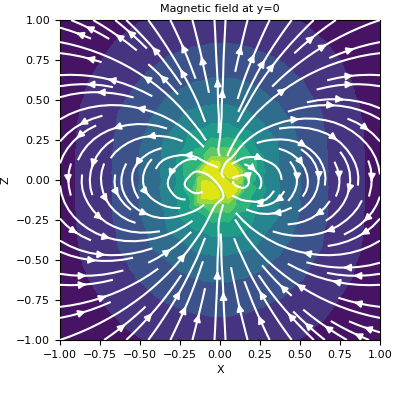