geoana.em.fdem.vertical_magnetic_field_horizontal_loop

geoana.em.fdem.vertical_magnetic_field_horizontal_loop(frequencies, sigma=1.0, mu=1.25663706212e-06, radius=1.0, current=1.0, turns=1, secondary=True)

Vertical magnetic field at the center of a horizontal loop for each frequency

Simple function to calculate the vertical magnetic field due to a harmonic horizontal loop. The anlytic form is only available at the center of the loop.

Parameters:

frequenciesfloat, or numpy.ndarray

frequencies in Hz

sigmafloat, complex, or numpy.ndarray, optional

electrical conductivity in S/m. Can provide a complex conductivity at each frequency if dispersive (i.e. induced polarization)

mufloat, complex, or numpy.ndarray, optional

magnetic permeability in H/m. Can provide a complex permeability at each frequency if dispersive (i.e. viscous remanent magnetization)

radiusfloat, optional

radius of the loop in meters

current: float, optional

transmitter current in A

turnsint, optional

number of turns for the loop source

secondarybool, optional

if True, the secondary field is returned. If False, the total field is returned. Default is True

Returns:

complex, or numpy.ndarray

The vertical magnetic field (H/m). If secondary is True, only the secondary field is returned. If secondary is False, the total field is returned.

Notes

The inputs values will be broadcasted together following normal numpy rules, and will support general shapes. Therefore every input, except for the secondary flag, can be arrays of the same shape.

The analytic expression for the total magnetic field from equation 4.94 in Ward and Hohmann 1988:

\[H_z = - \frac{I}{k^2 a^3}\left[3 - \left(3 + 3 i k a - k^2 a^2\right)e^{-i k a}\right]\]

Examples

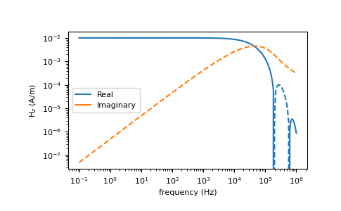
This example reproduces figure 4.7 from Ward and Hohmann

>>> import numpy as np
>>> import matplotlib.pyplot as plt
>>> from geoana.em.fdem import vertical_magnetic_field_horizontal_loop

Define the frequency range,

>>> frequencies = np.logspace(-1, 6, 200)
>>> hz = vertical_magnetic_field_horizontal_loop(frequencies, sigma=1E-2, radius=50, secondary=False)

Then plot the values

>>> plt.loglog(frequencies, hz.real, c='C0', label='Real')
>>> plt.loglog(frequencies, -hz.real, '--', c='C0')
>>> plt.loglog(frequencies, hz.imag, c='C1', label='Imaginary')
>>> plt.loglog(frequencies, -hz.imag, '--', c='C1')
>>> plt.xlabel('frequency (Hz)')
>>> plt.ylabel('H$_z$ (A/m)')
>>> plt.legend()
>>> plt.show()

(Source code, png, pdf)