geoana.em.static.ElectrostaticSphere.charge_density

ElectrostaticSphere.charge_density(xyz, dr=None)

charge density on the surface of a sphere in a uniform wholespace

Parameters:

xyz(…, 3) numpy.ndarray

Locations to evaluate at in units m.

drfloat, optional

Buffer around the edge of the sphere to calculate current density. Defaults to 5 % of the sphere radius

Returns:

rho: (…, ) np.ndarray

Examples

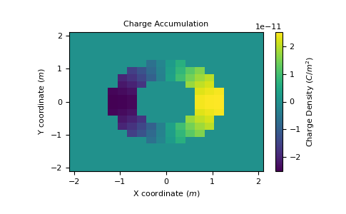
Here, we define a sphere with conductivity sigma_sphere in a uniform electrostatic field with conductivity sigma_background and plot the charge density.

>>> import numpy as np
>>> import matplotlib.pyplot as plt
>>> from matplotlib import patches
>>> from mpl_toolkits.axes_grid1 import make_axes_locatable
>>> from geoana.em.static import ElectrostaticSphere

Define the sphere.

>>> sigma_sphere = 10. ** -1
>>> sigma_background = 10. ** -3
>>> radius = 1.0
>>> simulation = ElectrostaticSphere(
>>>     location=None, sigma_sphere=sigma_sphere, sigma_background=sigma_background, radius=radius, primary_field=None
>>> )

Now we create a set of gridded locations and compute the charge density.

>>> X, Y = np.meshgrid(np.linspace(-2*radius, 2*radius, 20), np.linspace(-2*radius, 2*radius, 20))
>>> Z = np.zeros_like(X) + 0.25
>>> xyz = np.stack((X, Y, Z), axis=-1)
>>> q = simulation.charge_density(xyz, 0.5)

Finally, we plot the charge density.

>>> plt.pcolor(X, Y, q, shading='auto')
>>> cb1 = plt.colorbar()
>>> cb1.set_label(label= 'Charge Density ($C/m^2$)')
>>> plt.ylabel('Y coordinate ($m$)')
>>> plt.xlabel('X coordinate ($m$)')
>>> plt.title('Charge Accumulation')
>>> plt.show()

(Source code, png, pdf)