geoana.em.static.PointCurrentWholeSpace.current_density

PointCurrentWholeSpace.current_density(xyz)

Current density for a point current in a wholespace.

This method computes the curent density for the point current in a wholespace at the set of gridded xyz locations provided. Where \(\rho\) is the electric resistivity and \(\mathbf{E}\) is the electric field for the point current. The current density \(\mathbf{J}\) is:

\[\mathbf{J} = \frac{\mathbf{E}}{\rho}\]

Parameters:

xyz(…, 3) numpy.ndarray

Locations to evaluate at in units m.

Returns:

J(…, 3) np.ndarray

Current density of point current in units \(\frac{A}{m^2}\).

Examples

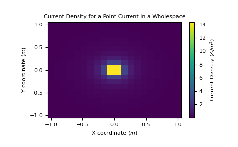
Here, we define a point current with current=1A in a wholespace and plot the current density.

>>> import numpy as np
>>> import matplotlib.pyplot as plt
>>> from geoana.em.static import PointCurrentWholeSpace

Define the point current.

>>> rho = 1.0
>>> current = 1.0
>>> simulation = PointCurrentWholeSpace(
>>>     current=current, rho=rho, location=None
>>> )

Now we create a set of gridded locations and compute the current density.

>>> X, Y = np.meshgrid(np.linspace(-1, 1, 20), np.linspace(-1, 1, 20))
>>> Z = np.zeros_like(X)
>>> xyz = np.stack((X, Y, Z), axis=-1)
>>> j = simulation.current_density(xyz)

Finally, we plot the curent density.

>>> j_amp = np.linalg.norm(j, axis=-1)
>>> plt.pcolor(X, Y, j_amp, shading='auto')
>>> cb1 = plt.colorbar()
>>> cb1.set_label(label= 'Current Density ($A/m^2$)')
>>> plt.ylabel('Y coordinate ($m$)')
>>> plt.xlabel('X coordinate ($m$)')
>>> plt.title('Current Density for a Point Current in a Wholespace')
>>> plt.show()

(Source code, png, pdf)