geoana.em.tdem.ElectricDipoleWholeSpace.magnetic_field_time_deriv

ElectricDipoleWholeSpace.magnetic_field_time_deriv(xyz)

Time-derivative of the magnetic field for the transient current dipole at a set of gridded locations.

For an electric current dipole oriented in the \(\hat{u}\) direction with dipole moment \(I ds\), this method computes the time-derivative of the transient magnetic field at the set of observation times for the gridded xyz locations provided.

The analytic solution is adapted from Ward and Hohmann (1988). For a transient electric current dipole oriented in the \(\hat{x}\) direction, the solution at vector distance \(\mathbf{r}\) from the current dipole is:

\[\frac{\partial \mathbf{h}}{\partial t} = - \frac{2 \, \theta^5 Ids}{\pi^{3/2} \mu \sigma} e^{-\theta^2 r^2} \big ( - z \, \mathbf{\hat y} + y \, \mathbf{\hat z} \big )\]

where

\[\theta = \Bigg ( \frac{\mu\sigma}{4t} \Bigg )^{1/2}\]

Parameters:

xyz(…, 3) numpy.ndarray

Gridded xyz locations

Returns:

(n_time, …, 3) numpy.ndarray of float

Time-derivative of the transient magnetic field at all times for the gridded locations provided.

Examples

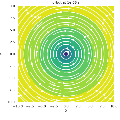
Here, we define a z-oriented electric dipole and plot the time-derivative of the magnetic field on the xy-plane that intercepts z=0.

>>> from geoana.em.tdem import ElectricDipoleWholeSpace
>>> from geoana.utils import ndgrid
>>> from geoana.plotting_utils import plot2Ddata
>>> import numpy as np
>>> import matplotlib.pyplot as plt

Let us begin by defining the electric current dipole.

>>> time = np.logspace(-6, -2, 3)
>>> location = np.r_[0., 0., 0.]
>>> orientation = np.r_[0., 0., 1.]
>>> current = 1.
>>> sigma = 1.0
>>> simulation = ElectricDipoleWholeSpace(
>>>     time, location=location, orientation=orientation,
>>>     current=current, sigma=sigma
>>> )

Now we create a set of gridded locations and compute the dh/dt.

>>> xyz = ndgrid(np.linspace(-10, 10, 20), np.linspace(-10, 10, 20), np.array([0]))
>>> dHdt = simulation.magnetic_field_time_deriv(xyz)

Finally, we plot dH/dt at the desired locations/times.

>>> t_ind = 0
>>> fig = plt.figure(figsize=(4, 4))
>>> ax = fig.add_axes([0.15, 0.15, 0.8, 0.8])
>>> plot2Ddata(xyz[:, 0:2], dHdt[t_ind, :, 0:2], ax=ax, vec=True, scale='log')
>>> ax.set_xlabel('X')
>>> ax.set_ylabel('Y')
>>> ax.set_title('dH/dt at {} s'.format(time[t_ind]))

(Source code, png, pdf)