geoana.em.static.DipoleHalfSpace.current_density

DipoleHalfSpace.current_density(xyz_m, xyz_n=None)

Current density for a dipole source in a halfspace.

This method computes the current density for a dipole source in a halfspace at

the set of gridded xyz locations provided. Where \(\rho\) is the electric resistivity and \(\mathbf{E}\) is the electric field for the dipole source. The current density \(\mathbf{J}\) is:

\[\mathbf{J} = \frac{\mathbf{E}}{\rho}\]

Parameters:

xyz_m(…, 3) numpy.ndarray

Location of the M voltage electrode.

xyz_n(…, 3) numpy.ndarray, optional

Location of the N voltage electrode.

Returns:

J(…, 3) np.ndarray

Current density of point current in units \(\frac{A}{m^2}\).

Examples

Here, we define a dipole source in a halfspace to compute current density.

>>> import numpy as np
>>> import matplotlib.pyplot as plt
>>> from mpl_toolkits.axes_grid1 import make_axes_locatable
>>> from geoana.em.static import DipoleHalfSpace

Define the dipole source.

>>> rho = 1.0
>>> current = 1.0
>>> location_a = np.r_[-1, 0, 0]
>>> location_b = np.r_[1, 0, 0]
>>> simulation = DipoleHalfSpace(
>>>     current=current, rho=rho, location_a=location_a, location_b=location_b
>>> )

Now we create a set of gridded locations and compute the current density.

>>> X, Y = np.meshgrid(np.linspace(-2, 2, 20), np.linspace(-2, 2, 20))
>>> Z = np.zeros_like(X)
>>> xyz = np.stack((X, Y, Z), axis=-1)
>>> j1 = simulation.current_density(xyz)
>>> j2 = simulation.current_density(xyz - np.r_[2, 0, 0], xyz + np.r_[2, 0, 0])

Finally, we plot the current density.

>>> fig, axs = plt.subplots(1, 2, figsize=(18,12))
>>> titles = ['3 Electrodes', '4 Electrodes']
>>> for ax, J, title in zip(axs.flatten(), [j1, j2], titles):
>>>     J_amp = np.linalg.norm(J, axis=-1)
>>>     im = ax.pcolor(X, Y, J_amp, shading='auto')
>>>     divider = make_axes_locatable(ax)
>>>     cax = divider.append_axes("right", size="5%", pad=0.05)
>>>     cb = plt.colorbar(im, cax=cax)
>>>     cb.set_label(label= 'Current Density ($A/m^2$)')
>>>     ax.streamplot(X, Y, J[..., 0], J[..., 1], density=0.75)
>>>     ax.set_ylabel('Y coordinate ($m$)')
>>>     ax.set_xlabel('X coordinate ($m$)')
>>>     ax.set_aspect('equal')
>>>     ax.set_title(title)

Finally, we plot the current density.

>>> J_amp = np.linalg.norm(j1, axis=-1)
>>> plt.pcolor(X, Y, J_amp, shading='auto')
>>> cb = plt.colorbar()
>>> cb.set_label(label= 'Current Density ($A/m^2$)')
>>> plt.streamplot(X, Y, j1[..., 0], j1[..., 1], density=0.75)
>>> plt.ylabel('Y coordinate ($m$)')
>>> plt.xlabel('X coordinate ($m$)')
>>> plt.title('Current Density from Dipole using 3 Electrodes')
>>> plt.tight_layout()
>>> plt.show()

(Source code, png, pdf)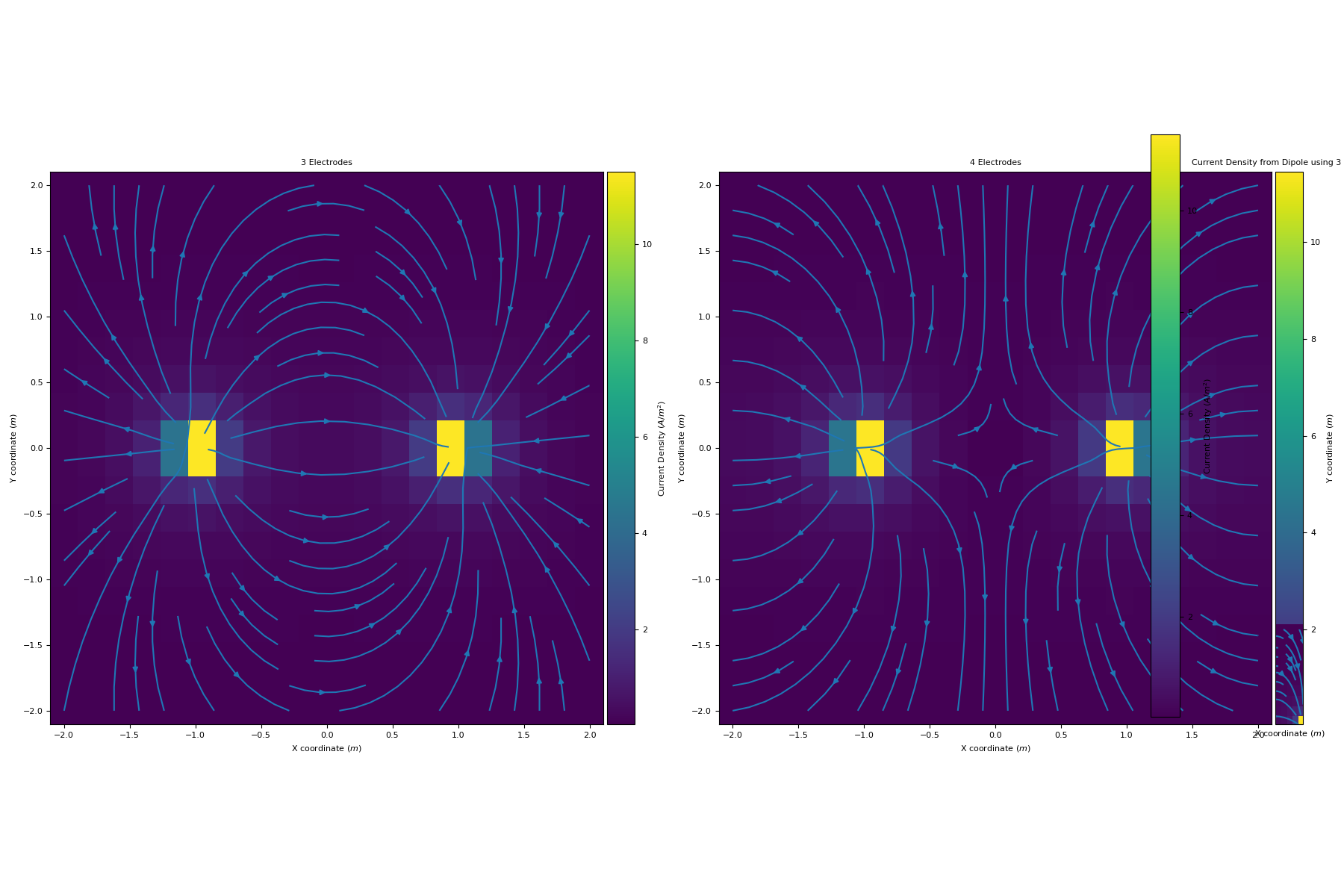