geoana.em.tdem.ElectricDipoleWholeSpace.vector_potential

ElectricDipoleWholeSpace.vector_potential(xyz)

Vector potential for the transient current dipole at a set of gridded locations.

For an electric current dipole oriented in the \(\hat{u}\) direction with dipole moment \(I ds\), this method computes the transient vector potential at the set of observation times for the gridded xyz locations provided.

The analytic solution is adapted from Ward and Hohmann (1988). For a transient electric current dipole oriented in the \(\hat{x}\) direction, the solution at vector distance \(\mathbf{r}\) from the current dipole is:

\[\mathbf{a}(t) = \frac{I ds}{4 \pi r} \, erf(\theta r) \, \hat{x}\]

where

\[\theta = \Bigg ( \frac{\mu\sigma}{4t} \Bigg )^{1/2}\]

Parameters:

xyz(n, 3) numpy.ndarray

Gridded xyz locations

Returns:

(n_time, n_loc, 3) numpy.array of float

Vector potential at all times for the gridded locations provided. Output array is squeezed when n_time and/or n_loc = 1.

Examples

Here, we define an x-oriented electric dipole and plot the vector potential on the xz-plane that intercepts y=0.

>>> from geoana.em.tdem import ElectricDipoleWholeSpace
>>> from geoana.utils import ndgrid
>>> from geoana.plotting_utils import plot2Ddata
>>> import numpy as np
>>> import matplotlib.pyplot as plt

Let us begin by defining the electric current dipole.

>>> time = np.logspace(-6, -2, 3)
>>> location = np.r_[0., 0., 0.]
>>> orientation = np.r_[1., 0., 0.]
>>> current = 1.
>>> sigma = 1.0
>>> simulation = ElectricDipoleWholeSpace(
>>>     time, location=location, orientation=orientation,
>>>     current=current, sigma=sigma
>>> )

Now we create a set of gridded locations and compute the vector potential.

>>> xyz = ndgrid(np.linspace(-10, 10, 20), np.array([0]), np.linspace(-10, 10, 20))
>>> E = simulation.vector_potential(xyz)

Finally, we plot the vector potential at the desired locations/times.

>>> t_ind = 0
>>> fig = plt.figure(figsize=(4, 4))
>>> ax = fig.add_axes([0.15, 0.15, 0.8, 0.8])
>>> plot2Ddata(xyz[:, 0::2], E[t_ind, :, 0::2], ax=ax, vec=True, scale='log')
>>> ax.set_xlabel('X')
>>> ax.set_ylabel('Z')
>>> ax.set_title('Vector potential at {} s'.format(time[t_ind]))

(Source code, png, pdf)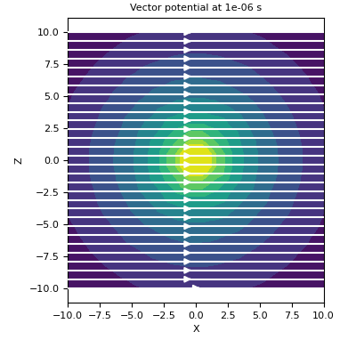