geoana.em.tdem.magnetic_field_time_deriv_magnetic_dipole

geoana.em.tdem.magnetic_field_time_deriv_magnetic_dipole(t, xy, sigma=1.0, mu=1.25663706212e-06, moment=1.0)

Magnetic field time derivative due to step off vertical dipole at the surface

Parameters:

t(n_t) numpy.ndarray

times (s)

xy(n_locs, 2) numpy.ndarray

surface field locations (m)

sigmafloat, optional

conductivity

mufloat, optional

magnetic permeability

momentfloat, optional

moment of the dipole

Returns:

dh_dt(n_t, n_locs, 3) numpy.ndarray

The magnetic field at the observation locations and times.

Notes

Matches the negative of equation 4.70 of Ward and Hohmann 1988, for the vertical component (due to the difference in coordinate sign conventionn used here).

\[\frac{\partial h_z}{\partial t} = \frac{m}{2 \pi \mu \sigma \rho^5}\left[ 9\mathrm{erf}(\theta \rho) - \frac{2\theta\rho}{\sqrt{\pi}}\left( 9 + 6\theta^2\rho^2 + 4\theta^4\rho^4\right) e^{-\theta^2\rho^2} \right]\]

Also matches equation 4.74 for the horizontal components

\[\frac{\partial h_\rho}{\partial t} = -\frac{m \theta^2}{2 \pi \rho t}e^{-\theta^2\rho^2/2} \left[ (1 +\theta^2 \rho^2) I_0 \left( \frac{\theta^2\rho^2}{2} \right) - \left( 2 + \theta^2\rho^2 + \frac{4}{\theta^2\rho^2}\right)I_1\left(\frac{\theta^2\rho^2}{2}\right) \right]\]

Examples

Reproducing the time derivate parts of Figure 4.4 and 4.5 from Ward and Hohmann 1988

>>> import numpy as np
>>> import matplotlib.pyplot as plt
>>> from geoana.em.tdem import magnetic_field_time_deriv_magnetic_dipole

Calculate the field at the time given, 100 m along the x-axis,

>>> times = np.logspace(-6, 0, 200)
>>> xy = np.array([[100, 0, 0]])
>>> dh_dt = magnetic_field_time_deriv_magnetic_dipole(times, xy, sigma=1E-2)

Match the vertical magnetic field plot

>>> plt.loglog(times*1E3, dh_dt[:,0, 2], c='C0', label=r'$\frac{\partial h_z}{\partial t}$')
>>> plt.loglog(times*1E3, -dh_dt[:,0, 2], '--', c='C0')
>>> plt.loglog(times*1E3, dh_dt[:,0, 0], c='C1', label=r'$\frac{\partial h_x}{\partial t}$')
>>> plt.loglog(times*1E3, -dh_dt[:,0, 0], '--', c='C1')
>>> plt.xlabel('time (ms)')
>>> plt.ylabel(r'$\frac{\partial h}{\partial t}$ (A/(m s))')
>>> plt.legend()
>>> plt.show()

(Source code, png, pdf)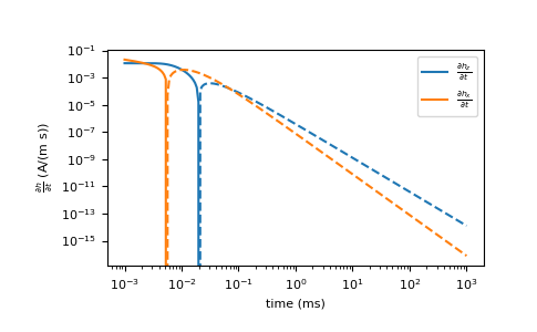