geoana.em.fdem.MagneticDipoleLayeredHalfSpace.magnetic_field

MagneticDipoleLayeredHalfSpace.magnetic_field(xyz, field='secondary')

Compute the magnetic field produced by a magnetic dipole over a layered halfspace.

Parameters:

xyznumpy.ndarray

receiver locations of shape (n_locations, 3). The z component cannot be below the surface (z >= 0.0).

field(“secondary”, “total”)

Flag for the type of field to return.

Returns:

(n_freq, n_loc, 3) numpy.array of complex

Magnetic field at all frequencies for the gridded locations provided. Output array is squeezed when n_freq and/or n_loc = 1.

Notes

We compute the magnetic using the Hankel transform solutions from Ward and Hohmann. For the vertical component of the magnetic dipole, the vertical and horizontal fields are given by equations 4.45 and 4.46:

\[H_\rho = \frac{m_z}{4\pi} \int_0^\infty \bigg [ e^{-u_0 (z - h)} - r_{te} e^{u_0 (z + h)} \bigg ] \lambda^2 J_1 (\lambda \rho) \, d\lambda\]

\[H_z = \frac{m_z}{4\pi} \int_0^\infty \bigg [ e^{-u_0 (z - h)} + r_{te} e^{u_0 (z + h)} \bigg ] \frac{\lambda^3}{u_0} J_0 (\lambda \rho) \, d\lambda\]

For the horizontal component of the magnetic dipole, we compute the contribution by adapting Ward and Hohmann equations 4.119-4.121; which is for an x-oriented magnetic dipole:

\[\begin{split}H_x = & -\frac{m_x}{4\pi} \bigg ( \frac{1}{\rho} - \frac{2x^2}{\rho^3} \bigg ) \int_0^\infty \bigg [ e^{-u_0 (z - h)} - r_{te} e^{u_0 (z + h)} \bigg ] \lambda J_1 (\lambda \rho) \, d\lambda \\ & -\frac{m_x}{4\pi} \frac{x^2}{\rho^2} \int_0^\infty \bigg [ e^{-u_0 (z - h)} - r_{te} e^{u_0 (z + h)} \bigg ] \lambda^2 J_0 (\lambda \rho) \, d\lambda\end{split}\]

\[\begin{split}H_y = & \frac{m_x}{2\pi} \frac{xy}{\rho^3} \int_0^\infty \bigg [ e^{-u_0 (z - h)} - r_{te} e^{u_0 (z + h)} \bigg ] \lambda J_1 (\lambda \rho) \, d\lambda \\ & -\frac{m_x}{4\pi} \frac{xy}{\rho^2} \int_0^\infty \bigg [ e^{-u_0 (z - h)} - r_{te} e^{u_0 (z + h)} \bigg ] \lambda^2 J_0 (\lambda \rho) \, d\lambda\end{split}\]

\[H_z = \frac{m_x}{4\pi} \frac{x}{\rho} \int_0^\infty \bigg [ e^{-u_0 (z - h)} + r_{te} e^{u_0 (z + h)} \bigg ] \lambda^2 J_1 (\lambda \rho) \, d\lambda\]

Examples

Here, we define an z-oriented magnetic dipole at (0, 0, 0) and plot the secondary magnetic field at multiple frequencies at (5, 0, 0). We compare the secondary fields for a halfspace and for a layered Earth.

>>> from geoana.em.fdem import (
>>>     MagneticDipoleHalfSpace, MagneticDipoleLayeredHalfSpace
>>> )
>>> from geoana.utils import ndgrid
>>> from geoana.plotting_utils import plot2Ddata
>>> import numpy as np
>>> import matplotlib.pyplot as plt

Let us begin by defining the electric current dipole.

>>> frequency = np.logspace(2, 6, 41)
>>> location = np.r_[0., 0., 0.]
>>> orientation = np.r_[0., 0., 1.]
>>> moment = 1.

We now define the halfspace simulation.

>>> sigma = 1.0
>>> simulation_halfspace = MagneticDipoleHalfSpace(
>>>     frequency, location=location, orientation=orientation,
>>>     moment=moment, sigma=sigma
>>> )

And the layered Earth simulation.

>>> sigma_top = 0.1
>>> sigma_middle = 1.0
>>> sigma_bottom = 0.01
>>> thickness = np.r_[5., 2.]
>>> sigma_layers = np.r_[sigma_top, sigma_middle, sigma_bottom]
>>> simulation_layered = MagneticDipoleLayeredHalfSpace(
>>>     frequency, thickness, location=location, orientation=orientation,
>>>     moment=moment, sigma=sigma_layers
>>> )

Now we define the receiver location and plot the seconary field.

>>> xyz = np.c_[5, 0, 0]
>>> H_halfspace = simulation_halfspace.magnetic_field(xyz, field='secondary')
>>> H_layered = simulation_layered.magnetic_field(xyz, field='secondary')

Finally, we plot the real and imaginary components of the magnetic field.

>>> fig = plt.figure(figsize=(6, 4))
>>> ax1 = fig.add_axes([0.15, 0.15, 0.8, 0.8])
>>> ax1.semilogx(frequency, np.real(H_halfspace[:, 2]), 'r', lw=2)
>>> ax1.semilogx(frequency, np.imag(H_halfspace[:, 2]), 'r--', lw=2)
>>> ax1.semilogx(frequency, np.real(H_layered[:, 2]), 'b', lw=2)
>>> ax1.semilogx(frequency, np.imag(H_layered[:, 2]), 'b--', lw=2)
>>> ax1.set_xlabel('Frequency (Hz)')
>>> ax1.set_ylabel('Secondary field (H/m)')
>>> ax1.grid()
>>> ax1.autoscale(tight=True)
>>> ax1.legend(['Halfspace: real', 'Halfspace: imag', 'Layered: real', 'Layered: imag'])

(Source code, png, pdf)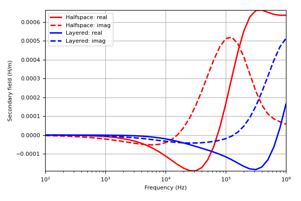